
📚 Machine Learning Series
1️⃣ Part 1: Supervised Learning & Neural Networks
2️⃣ Part 2: Randomized Optimization
3️⃣ Part 3: Unsupervised Learning & Dimensionality Reduction
4️⃣ (Coming soon)
In the primary Machine Learning course, we explored various algorithms via experimental analysis on two datasets — white wine and abalone. Below is an overview of my analysis on supervised learning algorithms.
Choosing Datasets
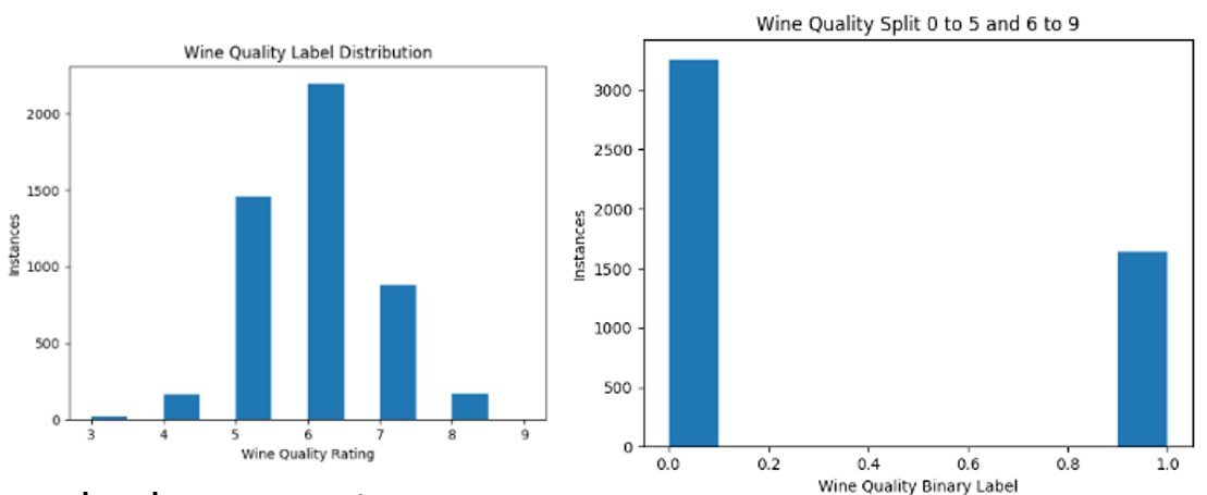
The popular wine quality score dataset I chose is based on a chemical analysis of wines grown in Italy — and the resulting user "quality" scores — scored from 0 to 10. Key attributes of the wine dataset include the amounts of:
alcohol, malic acid, magnesium, phenols, and flavonoids.
The idea of choosing a dataset like this is that it's a simple classification problem that's well-suited for determining if chemical constituents of wine can predict quality scores. The wine industry is worth billions in California alone, and if wine producers can find out what chemical constituents produce higher quality wines (at least in the minds of customers), then they likely will.
The other dataset I used was a modified version of the abalone age dataset — the idea being to predict the age of an abalone based on physical measurements such as:
length, diameter, shucked weight, and gender.
The actual age of the animal is determined by counting the numbers of rings — however, this is a time-consuming process that requires a microscope. Therefore, the goal of this dataset is to see if there's a better proxy attribute to use to count rings.
Algorithm Analysis
The code itself is basically searching all possible hyperparameters of each algorithm to find optimal results. I used sklearn's GridSearchCV function, which searches over a specified range of hyperparameters, finding the optimal hyperparameter combination. The code splits the data into a 70/30 train/test split, normalizes it to a standard scale, performs 5-fold cross-validation on the 70% training data for each hyperparameter combination, and finally calculates the average cross-validation score among the 5 folds. The best 5-fold cross-validation score from our grid search lets us know what the optimal hyperparameters are.
With the optimal hyperparameters, I can use these settings on the 30% held-out test set for each different supervised algorithm and determine which algorithm would perform the best for solving the central idea of each dataset (predicting quality or predicting age).
Supervised
In the supervised assignment, I looked at K-Nearest Neighbors, Decision Trees, Artificial Neural Networks, Boosting, and Support Vector Machines.
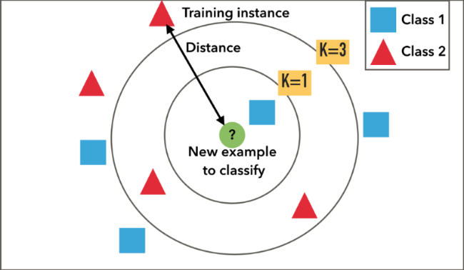
K-Nearest Neighbors (KNN)
KNN is a simple instance-based algorithm that simply looks at the k nearest points in feature space. For classification, this is simply a vote or choosing the mode of the neighbors' classes, whereas in a regression setting this would be the weighted mean. Some of the hyperparameters chosen for KNN include k, distance functions (Manhattan, Euclidean, and Chebyshev), and whether we weight each neighbor equally or by its distance to the point.
As seen in one of the convergence curves where the train and test were plotted against our value of k, we can see the bias-variance tradeoff at work. For low k values, we have a high variance situation with a highly complex model that only really works for training data — the model is not "general" enough. An intuitive way to think about this is if we have an outlier "good" wine classification in a normally "bad" wine region of space, if we have k=1, points around that outlier may be labeled incorrectly.
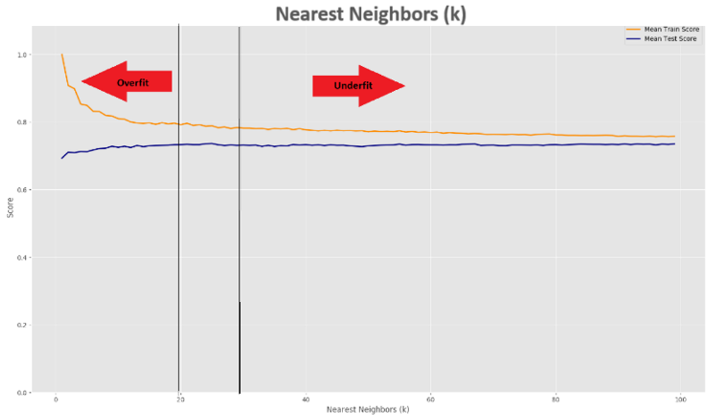
As we increase the value of k, it can be thought of as smoothing out the decision surface — which will decrease variance and increase bias. Increasing k too far leads to the opposite scenario — a high bias situation. It's all about finding the right balance point.
Decision Trees
In contrast to KNN, a decision tree is an eager learner as it builds the model on the training data first. Decision trees ask yes or no questions on features to determine which direction to branch. The final leaf node contains the prediction class. Decision trees work well with good splits of the data. In order to measure the quality of splits, I ran Entropy and Gini Index in the hyperparameter grid search. Some decision tree algorithms only look one move ahead to determine the current root of the tree — this is generally okay but usually not the most optimal. You usually want good splits at the top, which leads to shorter trees.
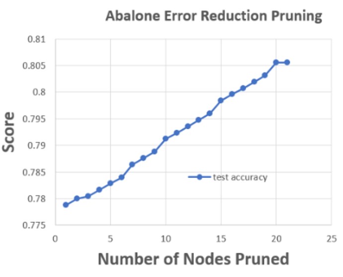
In some of the max depth experiments run, increasing the max depth leads to overfitting. If the tree is allowed too many nodes, it starts to exactly fit the training data — therefore it generalizes poorly for test data. Pruning or trimming nodes can help alleviate some of these overfitting issues. Error reduction pruning will attempt to remove the subtree at nodes, make them leaf and re-assign a class. If the resulting tree performs at least as well, that prune is kept. In both datasets, pruning boosted scores from about 75% to 80%.
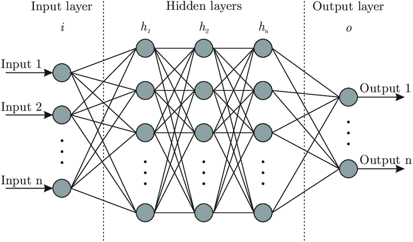
Artificial Neural Networks (ANN)
Artificial Neural Networks are learning algorithms modeled after brain neurons. The most basic unit is a perceptron that takes a weighted sum of inputs — if the sum is greater than some threshold (defined by the activation function), then that output is considered on or activated. ANN can tune the weight vectors (for each node connection) at each layer of the network by iteratively nudging them in small steps. The perceptron training rule will guarantee convergence (appropriate score/error) in a finite number of iterations if the data is linearly separable. Data that's not linearly separable will use the backpropagation rule and gradient descent to iteratively step down the gradient of the cost function. Issues can still occur, such as slow convergence or getting stuck in local minima.
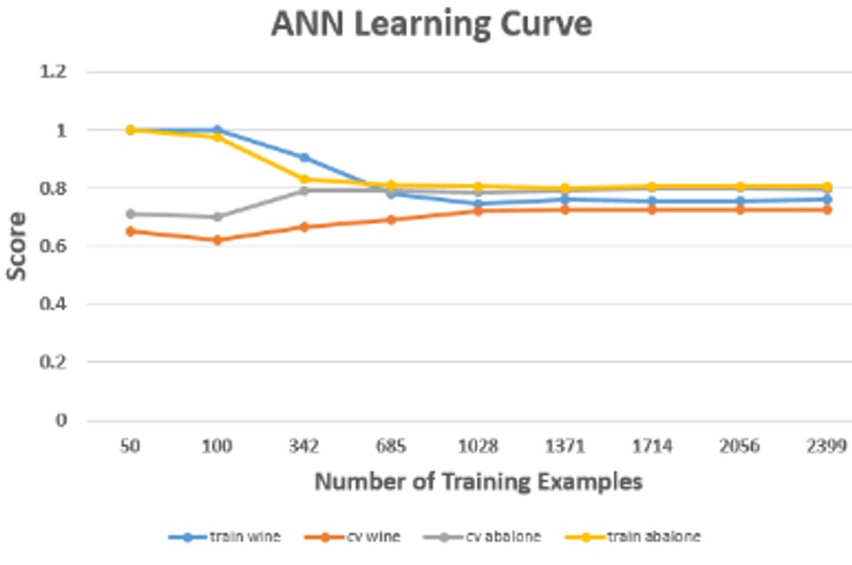
In my experiments, I used sklearn's MLPClassifier, which uses stochastic gradient descent — this looks at each training example individually to update weights, offering slightly better runtime than the alternative batch gradient descent.
Some of the experiments here included comparing some of the activation functions (logistic, relu, tanh, identity), comparing varying network dimensions (5, 10, 20 in the first layer versus 5, 10, or 20 in the second layer). Overall, ANN needs the fewest number of training examples of all the supervised algorithms to converge.
Boosting
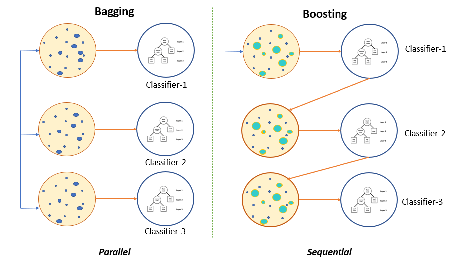
Boosting is an ensemble method of learning — the idea being combining many simple learners leads to a complex system that improves performance. In a common boosting algorithm like AdaBoost, each individual learner gets a weighted (depending on its error rate) vote towards the final hypothesis. In addition, each training example is given a variable weight. If the example is modeled poorly in previous learners, its weight increases; if it's modeled correctly, it decreases. Therefore, even with weak learners, we are always gaining information with learners. In general, boosting will reduce the bias (model complexity) in a model that's too general, whereas a related but different method, bagging, will reduce variance of a model that is too complex. Boosting can occasionally cause overfitting in a rare case where the first learner perfectly fits the training data, causing weights to never be updated.
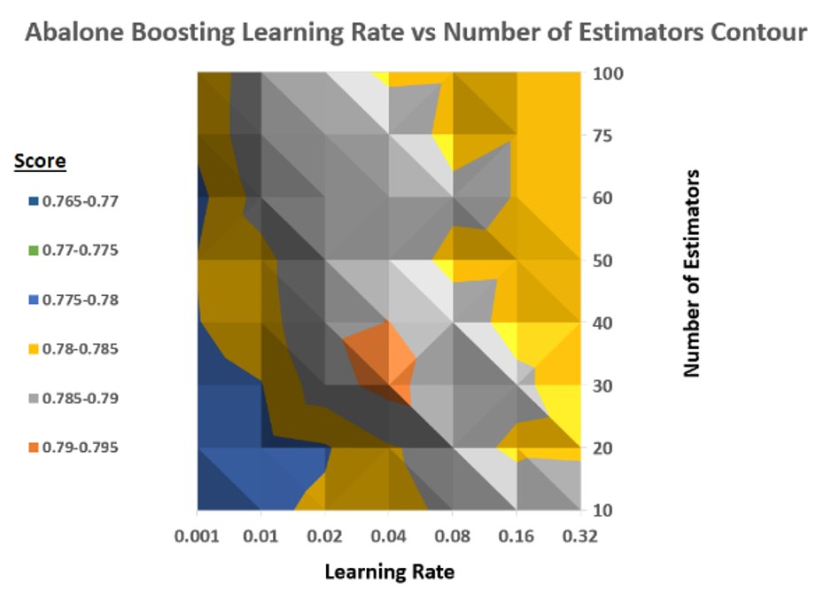
The experiments run on AdaBoost included varying number of estimators, varying learning rate, and comparing learning rate vs the number of estimators in 3D contour plots. AdaBoost has a default learning rate of 1 — however, this will slow down the adaptation of the model to training data. A max Abalone score around 30 estimators and a learning rate of 0.04 indicates that estimators have an equal voting power.
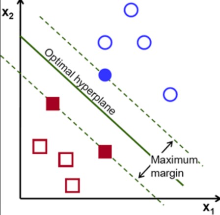
Support Vector Machines (SVM)
Support vector machines attempt to draw an optimal boundary that maximizes the margin width between different classes. Gutter lines define the max margin and go through points closest to the boundary. While ANN tries to reduce the error cost function, an SVM tries to maximize the margin while still classifying properly.
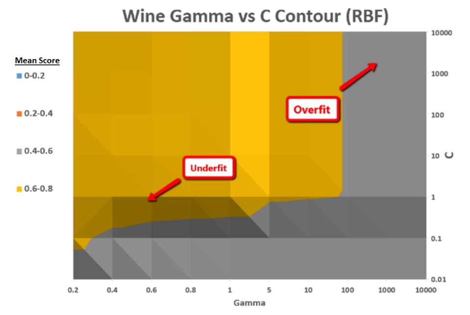
Using sklearn's support vector classifier, I plotted various hyperparameters including gamma (complexity of decision boundary), C (another parameter for decision boundary complexity), and several kernel functions (linear, rbf, poly).
One of the plots includes comparing gamma vs C on a contour plot with scores. Generally, a high gamma (like a low k in KNN) gives closer points more influence and creates a more complicated decision boundary. C acts similarly — a large value of C indicates a more complicated decision boundary. Often times the contour plots perfectly met intuition or expectations, but when I started plotting contour plots, it's sometimes tricky for them to exactly match expectations. That's true for the contour plot below — in general, the high value of these hyperparameters represents overfit areas, while the opposite corner represents underfit.
Comparison and Conclusion of Supervised Algorithms
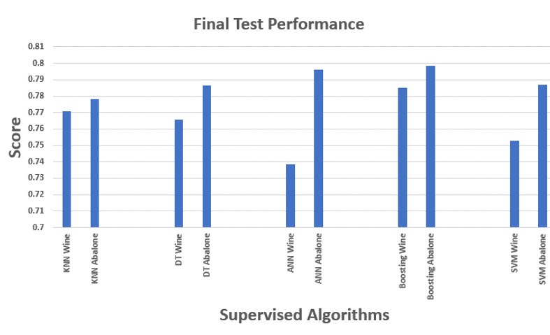
No final comparison is complete without consideration of both test performance and runtimes. Boosting was the clear winner and outperforms all other algorithms for both datasets. The only issue is if you look at time, AdaBoost performs the worst. KNN and Decision Trees run the fastest.
A key takeaway is the no free lunch theorem, which states that an algorithm effective for one problem may not be suitable for others. Each algorithm includes its own inductive biases and complexities. The only way to find the right tool for the job is to find the optimal hyperparameters and plot the performance — in addition to considering runtime performance.
Comparison Table
| Inductive Bias | Pros | Cons | Good at | |
|---|---|---|---|---|
| KNN | Classes are similar to nearest points | Intuitive; Fast runtime; Less prone to overfitting; Limited parameter tuning | Hard to model complex data; Lazy learner is slow to predict new instances; Poor on high dimensional datasets | Low-dimensional datasets |
| Decision Trees | Shorter trees preferred; High information gain splits at the top | Fast runtime; Robust to noise/missing values; Visually intuitive; Fast training & prediction | Possible duplication within tree; Complex trees can overfit and be hard to interpret | Medical diagnosis; Credit risk analysis |
| Artificial Neural Networks | Smooth interpolation; Bias towards minima via gradient descent | Can model complex relationships; Can separate signal from noise | Can overfit; Long training times; Black box; Many parameters | High dimensional datasets like images |
| Boosting (AdaBoost) | Ensembles reduce bias of individual learners | Flexible; Proven effective; Increases margin; Reduces overfitting | Weak classifiers too complex can overfit; Vulnerable to noise; Slow training | Problems with individual model instability |
| Support Vector Machines | Classes separated by wide margins | Can model complex relationships; Maximizing margins makes it robust to noise | Non-intuitive parameters; Long runtime; Not great for large or imbalanced datasets | Complex domains with clear margin or separation |
Future ML algorithm discussion coming...